Linear Algebra for Fun and Profit
Lecture 1 : 31 March 2020
Use PAGE DOWN and PAGE UP to go forwards and backwards
(You can also use the arrow keys, but that's more complicated. Hit ESC if you get lost!)
Introduction
This project is all about matrices and their applications. You have probably encountered matrices when solving systems of linear equations, such as the following:
$$ \begin{matrix} 2x & + & 4y & + & 2z & = & 16 \\ -2x & - & 3y & + & z & = & -5 \\ 2x & + & 2y & - & 3z & = & -3 \end{matrix} $$Such a system can be represented using matrices and vectors:
$$ \begin{pmatrix} 2 & 4 & 2 \\ -2 & -3 & 1 \\ 2 & 2 & -3 \end{pmatrix} \begin{pmatrix} x \\ y \\ z \end{pmatrix} = \begin{pmatrix} 16 \\ -5 \\ -3 \end{pmatrix} $$We may write this as an equation of the form $\mathbf{Ax} = \mathbf{b}$, where
$$ \mathbf{A} = \begin{pmatrix} 2 & 4 & 2 \\ -2 & -3 & 1 \\ 2 & 2 & -3 \end{pmatrix} , \quad \mathbf{x} = \begin{pmatrix} x \\ y \\ z \end{pmatrix} , \quad \mathbf{b} = \begin{pmatrix} 16 \\ -5 \\ -3 \end{pmatrix} $$Our goal is to solve for $\mathbf{x}$, given $\mathbf{A}$ and $\mathbf{b}$.
If we can find $\mathbf{A}^{-1}$ (the inverse of $\mathbf{A}$), then our solution $\mathbf{x}$ is given by $\mathbf{A}^{-1}\mathbf{b}$, since
$$ \mathbf{A}^{-1}\,\mathbf{b} = \mathbf{A}^{-1}(\mathbf{Ax}) = (\mathbf{A}^{-1}\mathbf{A})\mathbf{x} = \mathbf{x}. $$How can we compute $\mathbf{A}^{-1}$?
While there are formulas for inverting small matrices by hand, doing this is not practical for larger matrices. Instead, we will use the Python programming language as a calculator:
""" Python code """

import numpy as np

A = np.array([[ 2,  4,  2],
              [-2, -3,  1],
              [ 2,  2, -3]])

A_inv = np.linalg.inv(A)

print(A_inv)
Don't worry about the code for now. All you need to know is that the inverse of $\mathbf{A}$ has been computed (A_inv in the code above), and is given by:
Substituting this into our equation for $\mathbf{x}$, we get
$$ \mathbf{x} = \mathbf{A}^{-1}\, \mathbf{b} = \begin{pmatrix} 3.5 & 8 & 5 \\ -2 & -5 & -3 \\ 1 & 2 & 1 \end{pmatrix} \begin{pmatrix} 16 \\ -5 \\ -3 \end{pmatrix} = \begin{pmatrix} 1 \\ 2 \\ 3 \end{pmatrix}. $$Thus, $x=1, y=2, z=3$ solves our system of equations. (Verify this for yourself!)
Reviewing the steps
Let us identify the steps that we took to solve our system of equations:
We identified a matrix representation for our problem.
- In our case, we represented our system of equations using the matrix $\mathbf{A}$, the vectors $\mathbf{x}$ and $\mathbf{b}$, and the equation $\mathbf{Ax} = \mathbf{b}$.
We identified matrix concepts that were useful to our problem.
- In our case, we decided that the inverse of $\mathbf{A}$ would help us solve our problem.
We used a programming language to carry out computations involving these concepts.
- In our case, we used Python to compute the inverse of $\mathbf{A}$.
This was a simple example. But the same steps still hold for more advance applications.
Over the next few weeks, I will cover various matrix concepts and how to carry out computations in Python, but we won't do that today. For the rest of this lecture, I will just provide an overview of the many things that can be represented as matrices.
More than solving equations
The goal of this project is to convince you that matrices are for much more than solving systems of linear equations.
Over the next few slides, we will see some of these applications.
Don't worry about the details. We will go over each example slowly in the future. This is just a trailer!
Networks
A network is a collection of nodes connected by edges.
A network with $n$ nodes may be represented as an $n \times n$ matrix, where a $1$ indicates nodes that are connected by an edge.
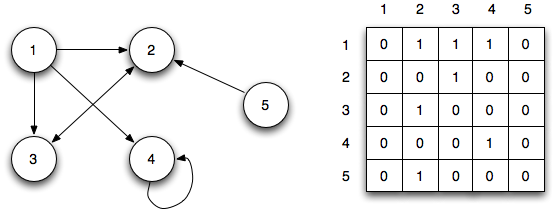
Networks can be used to represent many things:
- In a social network, nodes are people and we draw an edge between two people if they are friends with each other.
- In a ranking network, nodes could be football teams, and we draw an arrow from Team A to Team B if A defeated B in a match.
Google's PageRank algorithm uses a ranking network of webpages to decide which webpage is the most relevant to a search item.
Statistics
The correlation matrix shows statistical correlations between variables in a dataset.
For example, this matrix shows the correlations between properties of passengers on the Titanic:
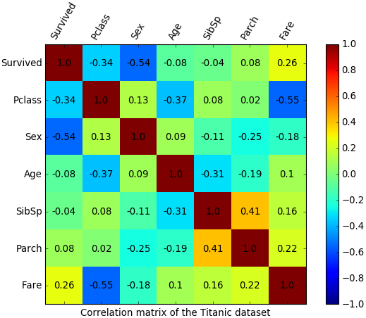
From this matrix, we see a positive correlation (0.26) between Fare and whether the passenger Survived!
Image processing
All digital images are matrices. Each entry of the matrix corresponds to one pixel.
By treating images as matrices, we can use matrix concepts to do things like image compression and image processing.
Dynamical systems
A dynamical system is anything that changes in a predictable manner over "time". In this example, time is discrete, and the graph shows the trajectory of a particle at each time step: (ignore the $x_1$ and $x_2$ labels. Treat them as the $x$- and $y$-axis instead.)

The system follows the matrix equation:
$$ \begin{pmatrix} x_{n+1} \\ y_{n+1} \end{pmatrix} = \begin{pmatrix} 1 & 1 \\ -1 & 1 \end{pmatrix}^n \begin{pmatrix} x_0 \\ y_0 \end{pmatrix} $$(In discrete systems, time is often represented by $n$ rather than $t$)
The Fibonacci series $0,1,1,2,3,5,8,\dots$ is also a discrete dynamical system. The system follows the matrix equation:
$$ \begin{pmatrix} F_n \\ F_{n+1} \end{pmatrix} = \begin{pmatrix} 0 & 1 \\ 1 & 1 \end{pmatrix}^n \begin{pmatrix} F_0 \\ F_1 \end{pmatrix} $$where $F_n$ denotes the $n^{th}$ Fibonacci number.
We will see how the matrix concept of eigenvalues helps us understand the long-term behaviour of such systems.
Equations in disguise
Sometimes, the solution to a problem may be found by solving a system of linear equations, but it may not be obvious that this is the case.
For example, the Lights-Out puzzle) actually involves solving a system of linear equations!
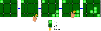
However, the entries of the matrices are not real numbers, but integers modulo 2. If time permits, we can investigate this as well.
Beyond linearity
The study of matrices is called linear algebra, and anything that can be solved with matrices is often described as being linear. However, there are plenty of non-linear problems out there.
Nevertheless, we will see that matrices are important in non-linear problems as well, such as in optimization and neural networks.
Homework
Write down (somewhere):
- Your name
- Why are you interested in this project?
- Among the topics listed today, which interests you the most?
- Which interests you the least?
Something to think about:
- Is there something you are interested in (e.g. your CCA, hobbies etc.) that can be represented with matrices?